pyfluentを使ったパラメトリック解析

By M.Sato

June 2, 2025

概要

pyfluentというpythonモジュールを使うことでpythonからfluentを実行可能であることは、以前のブログ記事においていくつか紹介した。

pyfluentは、現在活発に開発が進められておりgithubレポジトリを見るとほぼ毎日更新されていることがわかる。 pythonスクリプトの記述も徐々に洗練されて来ており、以前よりはかなり使いやすくなっている。

ここではpyfluentを使いパラメトリックに変数を変えて計算を行い、その結果に基づきエネルギー損失の応答曲面を作成した例を示す。

（注：現在、pyfluent-parametricのAPIは非推奨となっておりpyfluent-coreにその機能が含まれるようになっている。今回の解析ではpyfluentのパラメータ解析用のAPI(solver.settings.file.parametric_project)は使わないで python内で直接複数ケースの計算を行うようにした）

パラメトリック解析

２つの流入口から流入した流体が合流して一個の流出口から流出する流れ場を想定した。その際に流体エネルギーの損失が最も小さくなるようなケースを求めた。

解析モデル

代表的な形状(w1=0.01.w2=0.01)を使い解析モデルを示す。

図中の$w1,w2$がパラメータとなる寸法である。

２つの流入境界からの流入量はそれぞれ$0.05[kg/s]$であり、どの計算ケースでも同じとした。

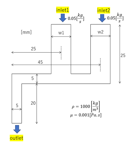
物性値

ここでは流体物性値を以下のように設定した。

密度: $\rho=1000[kg/m^3]$
粘度: $\mu=0.001[Pa.s]$

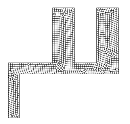
メッシュ作成

メッシュは、fluentに付属したメッシャーではなくgmsh(https://gmsh.info/)を使用して作成した。

２次元モデルであれば、簡単なgmshコマンドのスクリプトを記述すればfluentのライセンスを気にしないでメッシュを作成することができる。

なお、gmshから直接fluentで読み込み可能なメッシュは作成できないため、一度nastranのバルクデータ形式で出力し、その後、 fluentに読み込んで流体解析用に修正を行うようにした。

後述のpythonスクリプトにgmshをpythonから呼び出す関数（create_mesh()）を示している。 (流出入境界は形状作成で定義したcurveのタグ番号で区別している)。なおgmshは予めインストールしておく必要があることに注意。

作成したメッシュの例を示す。

目的関数の定義

機械エネルギーフラックス

流体の持っているエネルギーは流路を通過する際に低減する。

流出入境界における機械エネルギーフラックス(mechanical energy flux)を評価し、その差分が損失したエネルギーをみなして損失が最小となる条件を推定した。

$$ \begin{align} mechanical_energy_flux = \left( \frac{1}{2} v^2 + \frac{p}{\rho} \right) v_n \end{align} $$

ここで$v$は流速、$p$は圧力、$\rho$は密度である。

エネルギー損失

２つの流入境界と一個の流出境界における機械エネルギーフラックスを$Q_{in1},Q_{in2},Q_{out}$とし、次式で評価関数を定義した。これは全流入エネルギーと全流出エネルギーの差を全流入エネルギーで割り正規化したものになっている。この評価関数が小さいほど装置を通過する際のエネルギーの損失が小さいと考えることができる。

これを目的関数とした。

$$ \begin{align} objective_function = \frac{(Q_{in1}+Q_{in2}-Q_{out})}{Q_{in1}+Q_{in2}} \end{align} $$

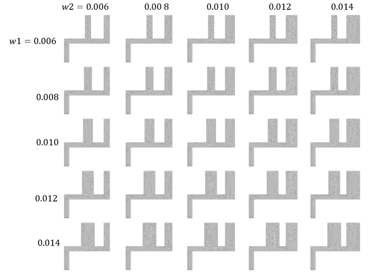
パラメータ空間

ここでは２つの流入境界の幅 $w1,w2$をパラメータとし、それぞれ以下の5個の値を取ることができるとした。なお実験計画法に基づき計算ケースを決めることも可能であるが、計算コストは微小であるため、ここでは全数を計算するようにした。従って全計算ケースは5x5=25である。各計算ケースのメッシュ分割を以下に示す。

    w1Arr = np.array([0.006, 0.008, 0.010, 0.012, 0.014])
    w2Arr = np.array([0.006, 0.008, 0.010, 0.012, 0.014])

解析結果

全ケースの計算を一括して実施する pythonスクリプト(response_surface.py)を作成し、計算を実施した。

各計算ケースの収束状況は自動的にログファイルに保存され、流出入境界におけるエネルギーフラックスはcsvファイルとして自動的に作成されるようにした。

今回の解析では全ての計算ケースが70回程度の反復回数で収束していることを確認した。

代表的な計算ケース($w1=0.01,w2=0.01$)の結果を示す。

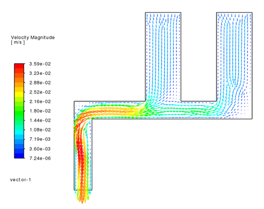流速ベクトル

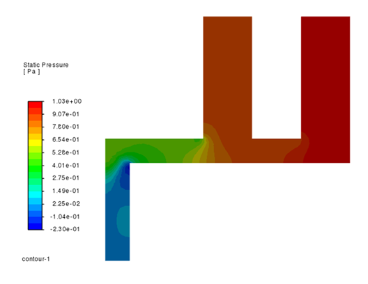圧力コンター

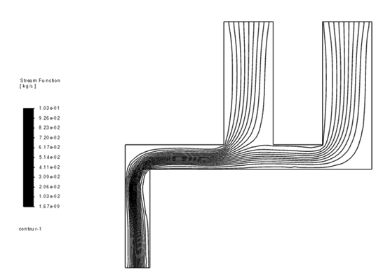流線

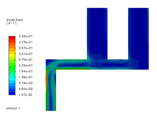せん断速度コンター（流路幅が小さい箇所でせん断速度大となる）

応答曲面

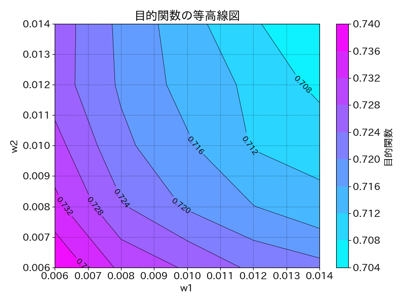
応答曲面（目的関数）のコンター図を作成するために plot_object.pyというpythonスクリプトを実行し、コンター図を作成した。

この応答曲面を見ると図の右上（w1=w2=0.014）においてエネルギー損失が最小となっていることがわかる。

エネルギー損失は粘性による摩擦力が流体粒子を変形させることが要因となっていると思われ、前出のせん断速度コンター図より、流入境界の流路幅が大きいほどエネルギー損失が小さくなっているものと推定される（エネルギー損失~せん断発熱~$せん断速度^2$）。

解析に使用したプログラム

以下に解析に使用したpythonスクリプトおよび目的関数の等高線をプロットするpythonスクリプトを示す。

パラメトリック解析用のスクリプト(response_surface.py)


import numpy as np
import ansys.fluent.core as pyfluent

#-----------------------------------------------------------------------------------
def create_mesh(c1,w1,c2,w2):
#-----------------------------------------------------------------------------------
    import gmsh

    lc = 0.001;

    x1, x2 = 0.00, 0.005
    x3 = c1 - w1/2.0
    x4 = c1 + w1/2.0
    x5 = c2 - w2/2.0
    x6 = c2 + w2/2.0

    y1, y2, y3, y4 = 0.00, 0.02, 0.025, 0.05

    gmsh.initialize()
    gmsh.model.add("mymesh")

    gmsh.model.geo.addPoint( x1 , y1, 0, lc,  1);
    gmsh.model.geo.addPoint( x2 , y1, 0, lc,  2);
    gmsh.model.geo.addPoint( x2 , y2, 0, lc,  3);
    gmsh.model.geo.addPoint( c1 , y2, 0, lc,  4);
    gmsh.model.geo.addPoint( x6 , y2, 0, lc,  5);
    gmsh.model.geo.addPoint( x6 , y4, 0, lc,  6);
    gmsh.model.geo.addPoint( x5 , y4, 0, lc,  7);
    gmsh.model.geo.addPoint( x5 , y3, 0, lc,  8);
    gmsh.model.geo.addPoint( x4 , y3, 0, lc,  9);
    gmsh.model.geo.addPoint( x4 , y4, 0, lc, 10);
    gmsh.model.geo.addPoint( x3 , y4, 0, lc, 11);
    gmsh.model.geo.addPoint( x3 , y3, 0, lc, 12);
    gmsh.model.geo.addPoint( x1 , y3, 0, lc, 13);

    gmsh.model.geo.addLine( 1, 2,11) # outlet
    gmsh.model.geo.addLine( 2, 3,12)
    gmsh.model.geo.addLine( 3, 4,13)
    gmsh.model.geo.addLine( 4, 5,14)
    gmsh.model.geo.addLine( 5, 6,15)
    gmsh.model.geo.addLine( 6, 7,16) # inlet2
    gmsh.model.geo.addLine( 7, 8,17)
    gmsh.model.geo.addLine( 8, 9,18)
    gmsh.model.geo.addLine( 9,10,19)
    gmsh.model.geo.addLine(10,11,20) # inlet1
    gmsh.model.geo.addLine(11,12,21)
    gmsh.model.geo.addLine(12,13,22)
    gmsh.model.geo.addLine(13, 1,23)

    gmsh.model.geo.addCurveLoop([11, 12, 13, 14, 15, 16, 17, 18, 19, 20, 21, 22, 23],1)
    gmsh.model.geo.addPlaneSurface([1], 1)
    
    gmsh.model.geo.mesh.setRecombine(2, 1)

    gmsh.model.geo.synchronize()
    gmsh.model.mesh.generate(2)

    gmsh.model.addPhysicalGroup(2,[1],1)  # solid
    gmsh.model.addPhysicalGroup(1,[11],2) # outlet
    gmsh.model.addPhysicalGroup(1,[20],3) # inlet1
    gmsh.model.addPhysicalGroup(1,[16],4) # inlet2

    gmsh.write("mymesh.bdf")
    gmsh.finalize()


#-----------------------------------------------------------------------------------
def run_fluent(c1,w1,c2,w2):
#-----------------------------------------------------------------------------------
    import ansys.fluent.core as pyfluent
    import subprocess

###########################################################################
# launch fluent, enable transcript file (trn), import bulkdata
# !caution! since overwriting of trn file is not allowed, they have to be removed beforehand

    solver = pyfluent.launch_fluent(
        precision="double",
        processor_count=1,
        version="2d"
    )
    print(solver.get_fluent_version())

    # import bulk data
    solver.tui.file.import_.nastran.bulkdata("mymesh.bdf")

    trnfile = 'case-{0}-{1}.trn'.format(w1,w2)
    solver.tui.file.start_transcript(trnfile)

    solver.settings.setup.models.energy = {"enabled": False}

    solver.settings.setup.models.viscous.model = "laminar"

###########################################################################
# create material property

    solver.settings.setup.materials.fluid["water"] = {
        "density": {"option": "constant", "value": 1000},
        "viscosity": {"option": "constant","value": 0.001  },
    }


###########################################################################
# adjust mesh data so fluid analysis can be performed

    # continuum cells are supposed as solid when imported, change to fluid
    solver.settings.setup.cell_zone_conditions.set_zone_type(
        zone_list=["solid-1"], new_type="fluid"
    )

    # change boundary name so human can identify easily
    solver.settings.setup.boundary_conditions.wall["wall-11"].rename("outlet")
    solver.settings.setup.boundary_conditions.wall["wall-20"].rename("inlet1")
    solver.settings.setup.boundary_conditions.wall["wall-16"].rename("inlet2")

    # change boundary type from "wall" to anything appropriate
    solver.settings.setup.boundary_conditions.set_zone_type(
        zone_list=["inlet1","inlet2"], new_type="mass-flow-inlet"
    )
    solver.settings.setup.boundary_conditions.set_zone_type(
        zone_list=["outlet"], new_type="pressure-outlet"
    )

    # assign fluid property to cell zone
    solver.settings.setup.cell_zone_conditions.fluid["fluid-1"].material = "water"

    # set boundary conditions
    inlet1 = solver.settings.setup.boundary_conditions.mass_flow_inlet["inlet1"]
    inlet1.momentum.mass_flow_rate.value = 0.05

    inlet2 = solver.settings.setup.boundary_conditions.mass_flow_inlet["inlet2"]
    inlet2.momentum.mass_flow_rate.value = 0.05

    outlet = solver.settings.setup.boundary_conditions.pressure_outlet["outlet"]

###############################################################################
# named expression to calculate mechanical energy flux

    solver.settings.setup.named_expressions["ene"] = {
        "definition": "StaticPressure/Density+Velocity.mag**2/2"
    }

###############################################################################
# solution methods

    solver.settings.solution.methods.p_v_coupling.flow_scheme = "SIMPLEC"
    solver.settings.solution.methods.spatial_discretization.discretization_scheme[
        "pressure"
    ] = "presto!"

###############################################################################
# Initialize flow field

    solver.settings.solution.initialization.initialization_type = "standard"
    solver.settings.solution.initialization.standard_initialize()

###############################################################################
# Solve for 300 iterations

    solver.solution.run_calculation.iterate(iter_count=300)
    file = 'case-{0}-{1}.cas.h5'.format(w1,w2)

    # save calculation result
    solver.settings.file.write_case_data(file_name=file)

    # calculate report
    ein1 = solver.scheme_eval.exec(
        ('(ti-menu-load-string "/report/surface-integrals/flow-rate inlet1 () expr:ene no")',)
    ).split(" ")[-1]
    ein2 = solver.scheme_eval.exec(
        ('(ti-menu-load-string "/report/surface-integrals/flow-rate inlet2 () expr:ene no")',)
    ).split(" ")[-1]
    eout = solver.scheme_eval.exec(
        ('(ti-menu-load-string "/report/surface-integrals/flow-rate outlet () expr:ene no")',)
    ).split(" ")[-1]

    dummy = solver.scheme_eval.exec(
        ('(ti-menu-load-string "/report/surface-integrals/area-weighted-avg inlet1 inlet2 outlet () pressure no")',)
    )
    dummy = solver.scheme_eval.exec(
        ('(ti-menu-load-string "/report/surface-integrals/area-weighted-avg inlet1 inlet2 outlet () velo-mag no")',)
    )
    dummy = solver.scheme_eval.exec(
        ('(ti-menu-load-string "/report/fluxes/mass-flow no inlet1 inlet2 outlet () no")',)
    )

    print('ein1={} ein2={} eout={}'.format(ein1,ein2,eout))

    solver.tui.file.stop_transcript()
    solver.exit()

    return ein1,ein2,eout


#-----------------------------------------------------------------------------------
def parametric_survey():
#-----------------------------------------------------------------------------------

    w1Arr = np.array([0.006, 0.008, 0.010, 0.012, 0.014])
    w2Arr = np.array([0.006, 0.008, 0.010, 0.012, 0.014])

    ein1Arr = np.zeros((w1Arr.shape[0], w2Arr.shape[0]))
    ein2Arr = np.zeros((w1Arr.shape[0], w2Arr.shape[0]))
    eoutArr = np.zeros((w1Arr.shape[0], w2Arr.shape[0]))

    for idx1, w1 in np.ndenumerate(w1Arr):
        for idx2, w2 in np.ndenumerate(w2Arr):

            create_mesh(0.025,w1,0.045,w2)

            ein1,ein2,eout = run_fluent(0.025,w1,0.045,w2)

            ein1Arr[idx1][idx2] = float(ein1)
            ein2Arr[idx1][idx2] = float(ein2)
            eoutArr[idx1][idx2] = -float(eout)

    with open("inlet1.csv","w") as o:
        for row in ein1Arr:
            o.write(",".join(map(str, row)) + "\n") 

    with open("inlet2.csv","w") as o:
        for row in ein2Arr:
            o.write(",".join(map(str, row)) + "\n") 

    with open("outlet.csv","w") as o:
        for row in eoutArr:
            o.write(",".join(map(str, row)) + "\n") 



if __name__ == "__main__":
    parametric_survey()

目的関数の等高線をプロットするスクリプト(plot_object.py)


import csv
import numpy as np
import matplotlib.pyplot as plt
import japanize_matplotlib

w1Arr = np.array([0.006, 0.008, 0.010, 0.012, 0.014])
w2Arr = np.array([0.006, 0.008, 0.010, 0.012, 0.014])

xval = np.zeros((w1Arr.shape[0], w2Arr.shape[0]))
yval = np.zeros((w1Arr.shape[0], w2Arr.shape[0]))
zval = np.zeros((w1Arr.shape[0], w2Arr.shape[0]))

with open('inlet1.csv') as f:
    reader = csv.reader(f)
    ein1 = [[float(cell) for cell in row] for row in reader]

with open('inlet2.csv') as f:
    reader = csv.reader(f)
    ein2 = [[float(cell) for cell in row] for row in reader]

with open('outlet.csv') as f:
    reader = csv.reader(f)
    eout = [[float(cell) for cell in row] for row in reader]


for i in range(len(eout)):
    for j in range(len(eout[0])):
        xval[i][j] = w1Arr[i]
        yval[i][j] = w2Arr[j]
        zval[i][j] = (ein1[i][j] + ein2[i][j] - eout[i][j])/(ein1[i][j] + ein2[i][j])
#       print(f"zval[{i}][{j}] = {zval[i][j]}")

##################################################################################

plt.rcParams['font.size'] = 14 # グラフの基本フォントサイズの設定

# タイトル名
my_title = f'目的関数の等高線図'

# グラフサイズ
plt.figure(figsize=(8, 6))  # 幅8インチ、高さ6インチ

# 等高線図のプロット
my_split = 10
contour = plt.contour(xval, yval, zval, levels=my_split, linewidths=0.5, colors='k')
contourf = plt.contourf(xval, yval, zval, levels=my_split, cmap='cool')  # カラーマップ

# 等高線上に数値をテキストで表示
plt.clabel(contour, inline=True, fontsize=11)  # fontsizeを変更

# 軸ラベルの設定
plt.xlabel(f'w1', fontsize=14)
plt.ylabel(f'w2', fontsize=14)

# タイトル
plt.title(my_title)

# カラーバーの追加
plt.colorbar(label="目的関数")

# 薄い点線のグリッドを追加
plt.grid(linestyle='dotted', alpha=0.5, color='k')

# レイアウトを調整
plt.tight_layout()

# グラフの表示
plt.show()

# グラフを画像ファイルで保存
#plt.savefig(f'contour.png')

まとめ

pyfluentを使いパラメトリック解析を行う例を示した。

メッシュ作成、解析の実行を自動的に行うことで効率よくパラメータの調査、応答曲面の作成を行うことができることがわかった。

弊社の解析事例

弊社の流体解析事例については、下記のリンクからご覧ください．

👉 解析事例のご紹介 FLUENT

👉 流体解析実績及び事例